


About
The Crop Haplotypes website provides an interactive graphic visualisation of the shared haplotypes between the wheat genome assemblies generated as part of the 10+ Wheat Genome Project (Brinton et al, 2020; Walkowiak et al, 2020).
We used chromosome-level genome assemblies of nine wheat cultivars (ArinaLrFor, Jagger, Julius, Lancer, Landmark, Mace, Norin61, Stanley, SY-Mattis) and the Chinese Spring RefSev1.0 assembly alongside scaffold-level assemblies of five additional cultivars (Cadenza, Claire, Paragon, Robigus and Weebill). For more details on the cultivars and overall context of the project see this link and the manuscript describing these assemblies (Walkowiak et al, 2020).
To call haplotype blocks we used a combination of whole chromosome level NUCmer alignments and gene-based pairwise alignments using BLASTn. Briefly, we defined haplotype blocks as physical regions with ≥99.99% sequence identity (across a fixed bin size of 5-, 2.5- or 1-Mbp) between pairwise comparisons of cultivars in the 10+ Wheat Genome Project. More details on this haplotype analysis and the underlying methodologies can be found in the manuscript "A haplotype-led approach to increase the precision of wheat breeding" (Brinton et al, 2020).
How to use the website
To search the website the user must first select the chromosome that they would like to examine.
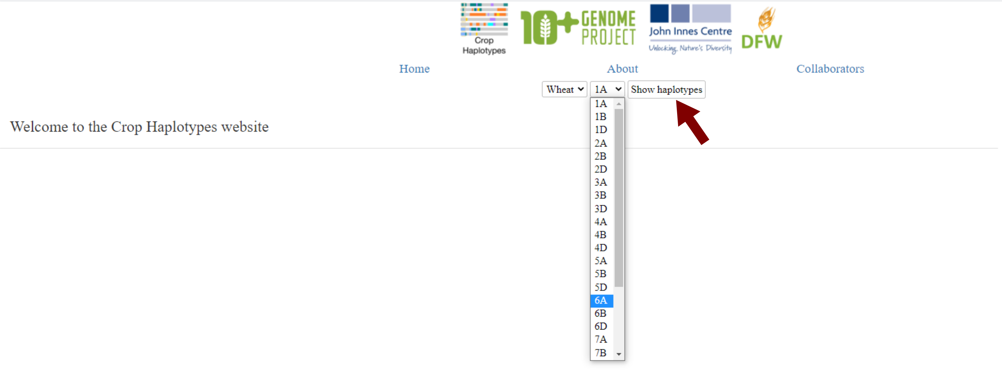
Once loaded, the visualisation displays the selected chromosome from all 15 cultivars using each cultivar’s own coordinate system as the x-axis (the exact length of each chromosome varies slightly between cultivars). At any given position, regions with the same colour share a common haplotype (i.e. identical-by-state sequence) as determined by the haplotype calling analysis described above (except for light grey regions which are not contained within haplotype blocks; i.e. they are unique to that cultivar in this analysis).
In the default view, all haplotype blocks shared amongst the 15 cultivars are displayed.
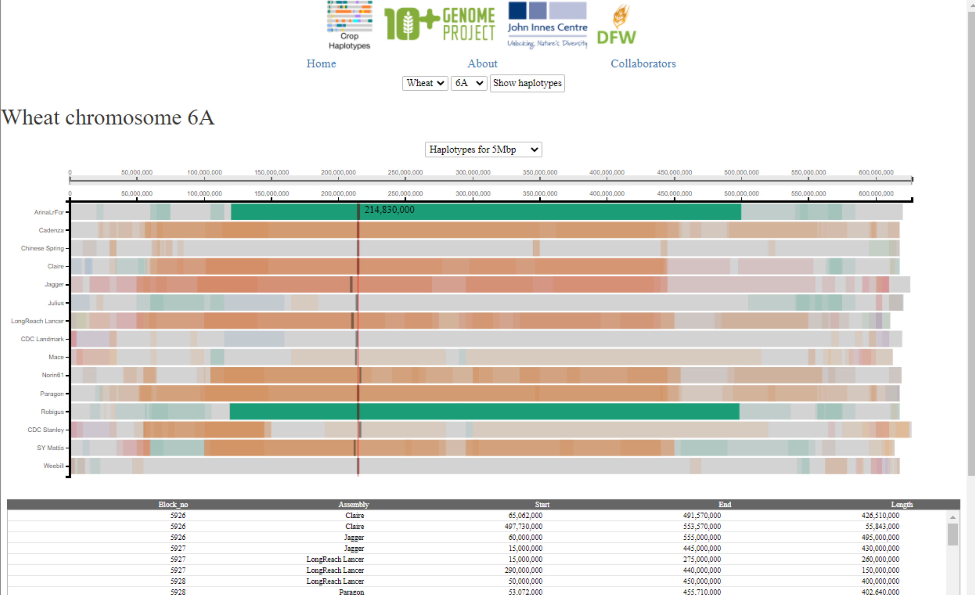
The user can hover the cursor over any block/position in the visualisation. This will highlight the individual haplotype block in the cultivar the cursor is hovering over, and the same block in any other culitvars that carry the same haplotype. This is indicated by the blocks remaining in block colour, whilst all other haplotype blocks are faded. The red line and number indicate the base-pair position of the cursor in the cultivar selected, whilst the dark grey lines that appear indicate the corresponding base-pair position in the other cultivars. This correspondence between genomic positions in different cultivars is based on a method using projections of the RefSeqv1.1 gene models to all assembiles (see Brinton et al, 2020 for full methods). As the user moves the cursor across the visualisation, different haplotype blocks will be highlighted and un-highlighted according to the cursor position.
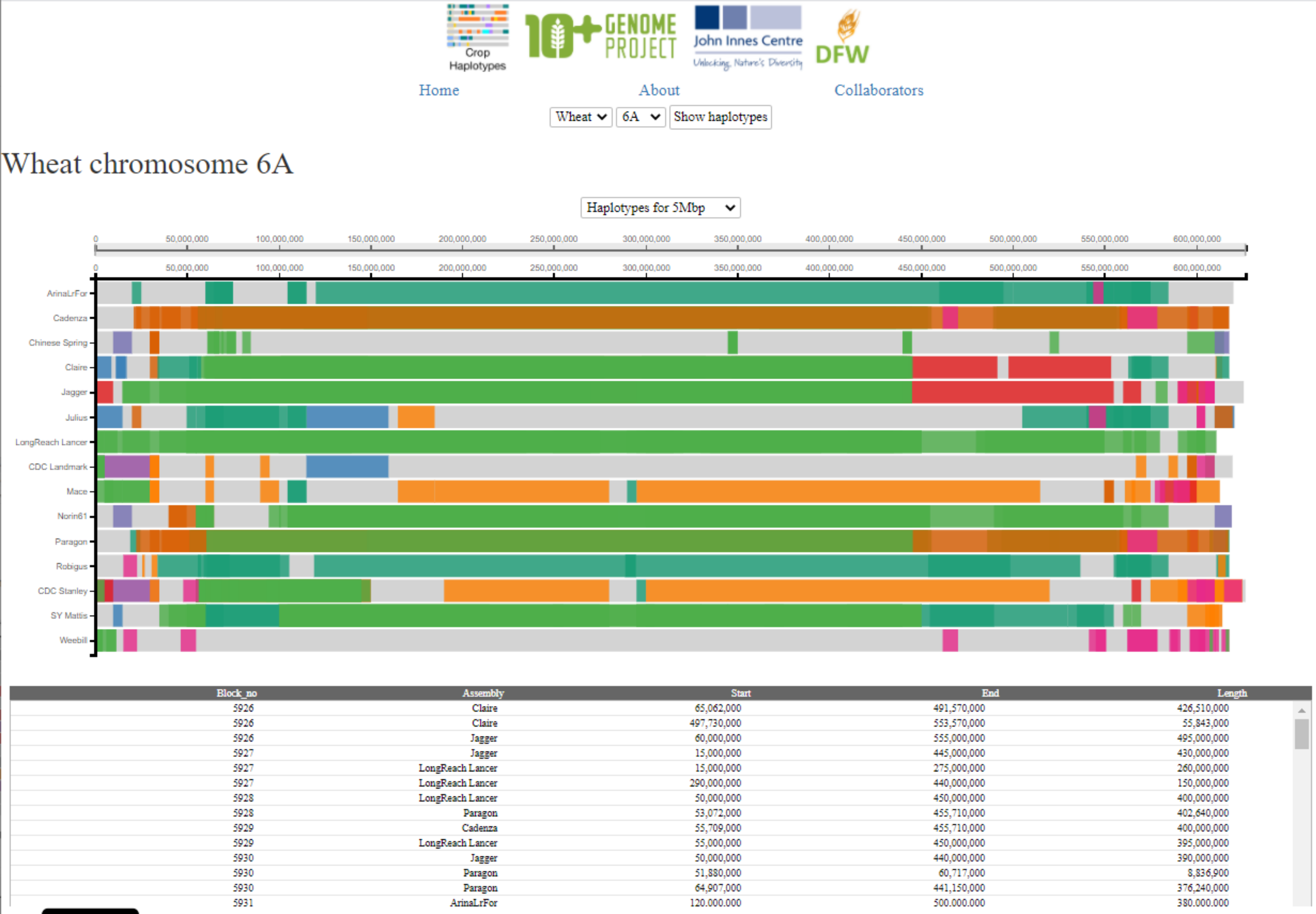
If the user clicks on a particular block then the position is fixed and the coordinates of the selected haplotype blocks will be displayed in the table below the visualisation. If the user clicks again, the previous behaviour of hovering over different blocks is resumed. By default (before clicking) the table below shows coordinates of all haplotype blocks on the selected chromosome. The table ccontains the following columns:
- Block_no: Each pairwise-haplotype block is given a unique numeric identifier
- Assembly: The name of the assembly (i.e. line or cultivar) to which the row corresponds (each block will have at least two entries in the table, one for each assembly/cultivar in the pairwise comparison)
- Start: Start coordinate in base-pairs of the haplotype block in the assembly to which the row corresponds
- End: End coordinate in base-pairs of the haplotype block in the assembly to which the row corresponds
- Length: The length of the haplotype block in base pairs in the assembly to which the row corresponds
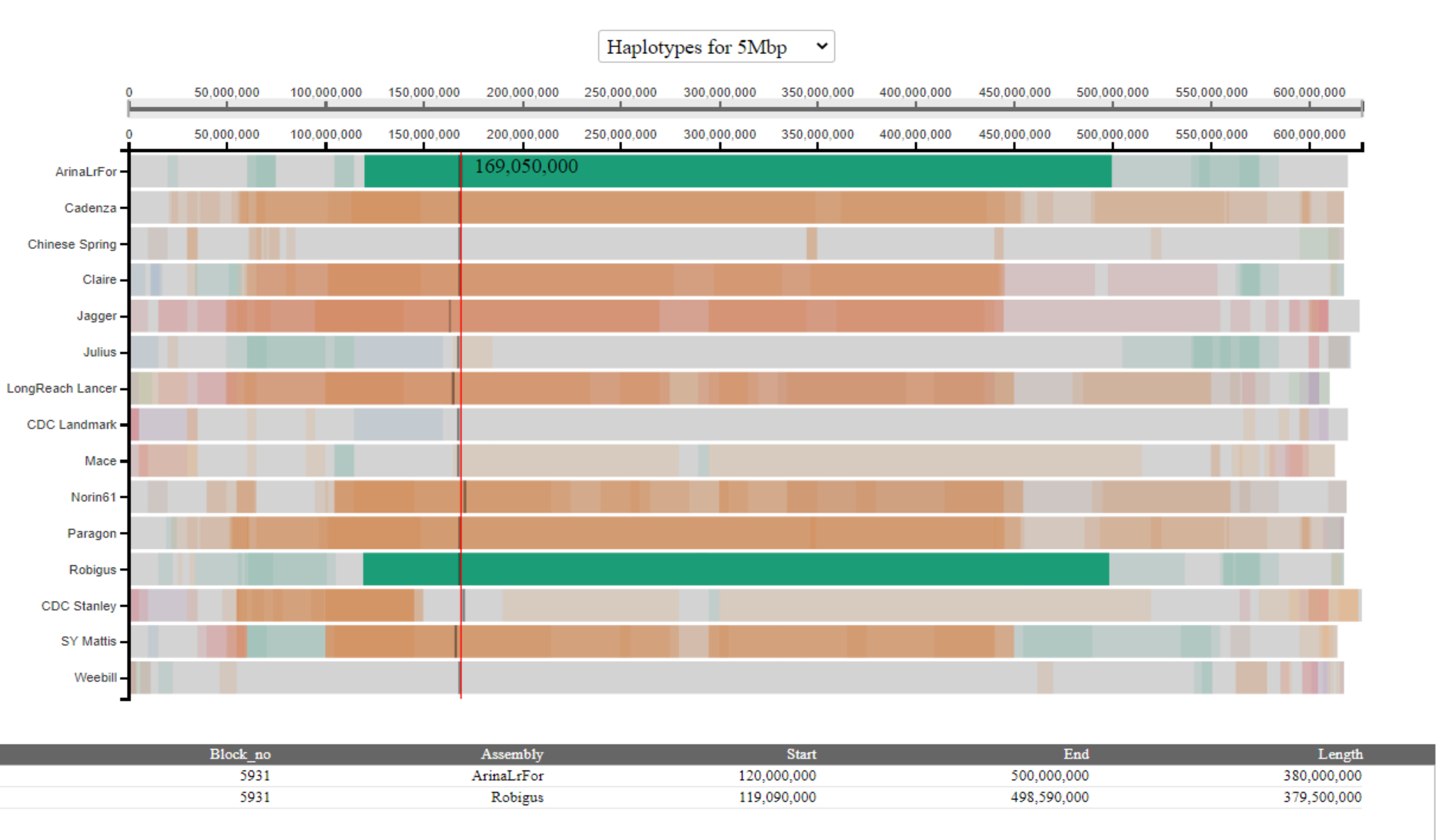
In the above example, we see that the selected haplotype block has two entries in the table; one corresponding to the coordinates in each of the cultivars carrying the block (in this example, Arina*LrFor* and Robigus).
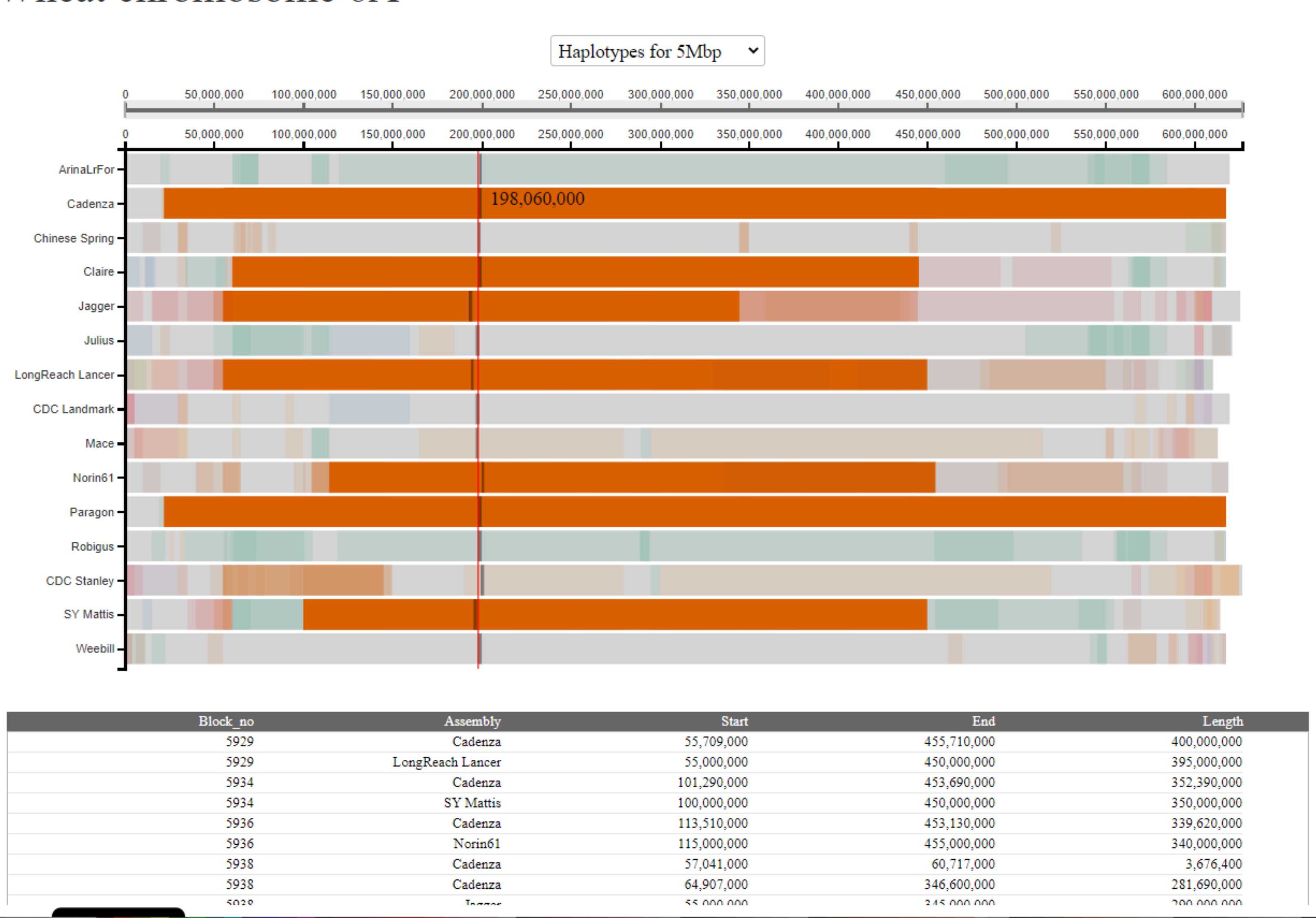
However, in other cases the table will contain more rows. This could be because more than two cultivars carry the haplotype block. In this case there will be rows giving details of the coordinates for all the pairwise comparisons it appears in. Importantly, the block will be given a different numeric identifier for each pairwise comparison it appears in e.g. in the example below we see that the selected block is given the identifier "5929" in the pairwise comparison between Cadenza and LongReach Lancer, but "5934" in the pairwise comparison between Cadenza and SY Mattis. This reflects the pairwise nature of the analysis.
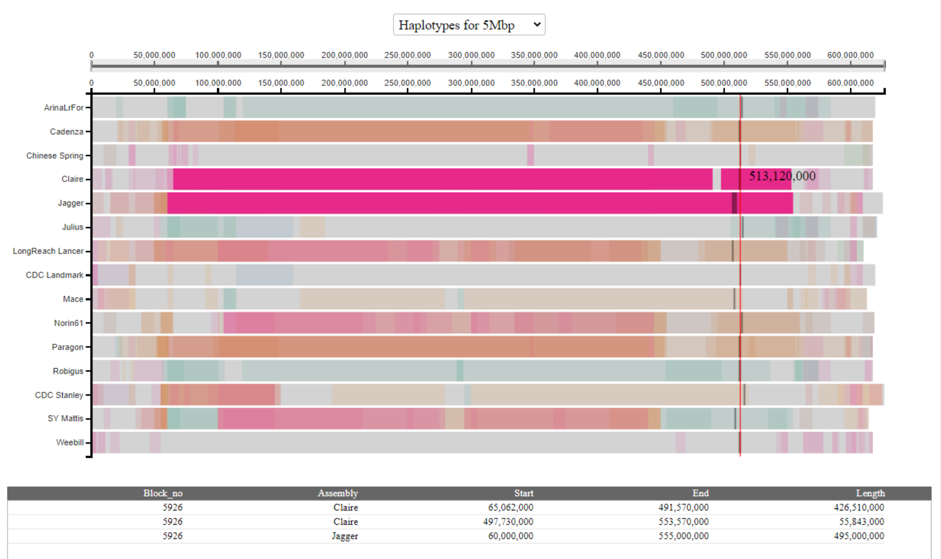
In other cases, there may be more than two rows with the same numeric identifier. This indicates cases where the haplotype block may be fragmented in one or both of the assemblies. In most cases these are likely to be technical artefacts arising as a result of the between-assembly coordinate conversion, or gaps in particular assemblies. If users are interested in fully understanding specific haplotype blocks they should manually inspect the alignments (all available at this link). In the example below, we see that the haplotype block is fragmented in the Claire assembly.
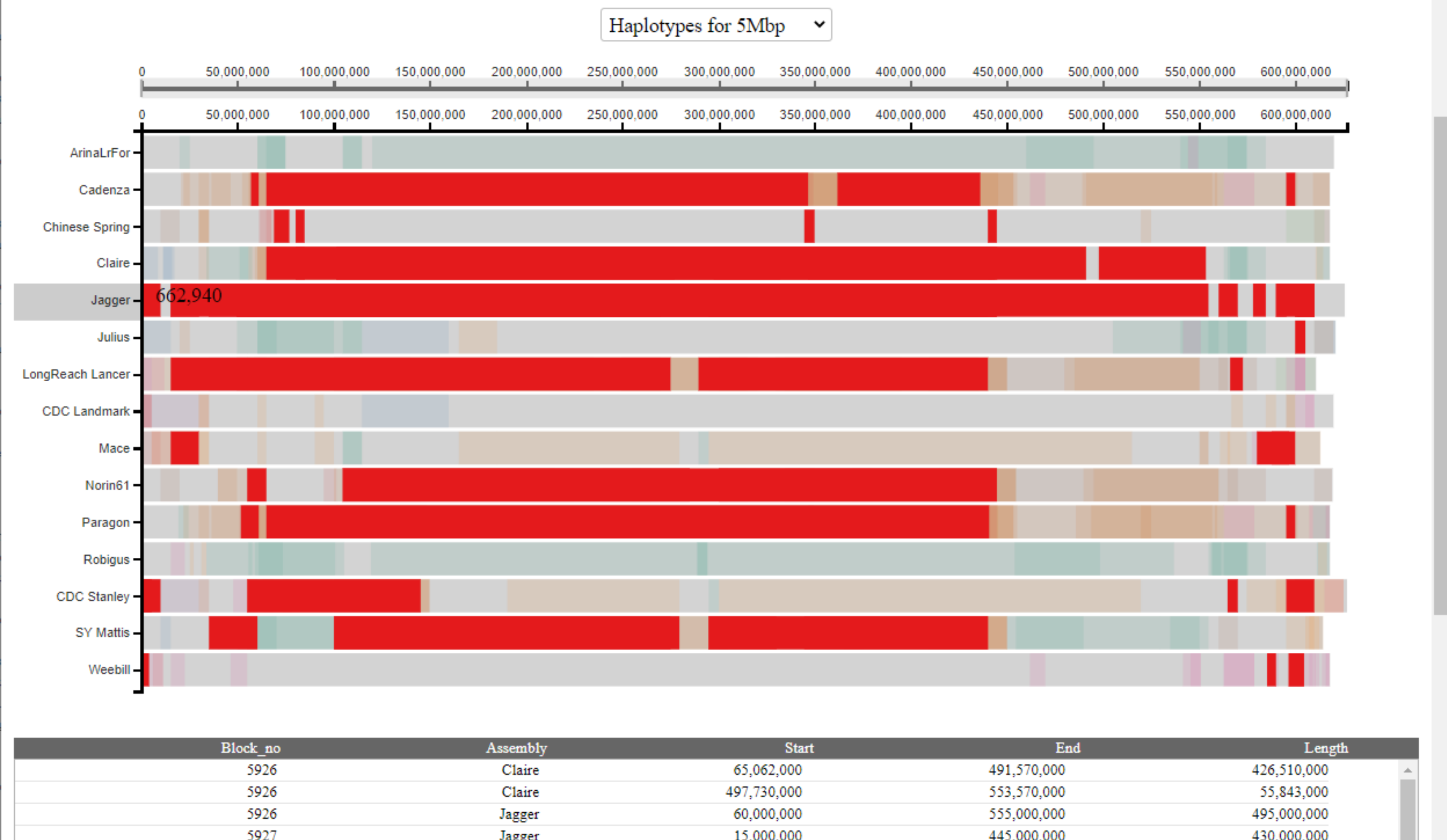
To view all haplotype blocks shared with a specific cultivar, the user can click on the name of the cultivar on the left-hand side. All haplotype blocks shared with this cultivar will be highlighted across all cultivars in a single colour and coordinates displayed in the table. In the example below, we highlight all haplotype blocks shared with Jagger:
The user may also highlight specific haplotype blocks based on the table by clicking rows of interest. Selected rows will be highlighted in black and multiple blocks can be selected and highlighted at the same time. The user can de-select rows by clicking on them again.
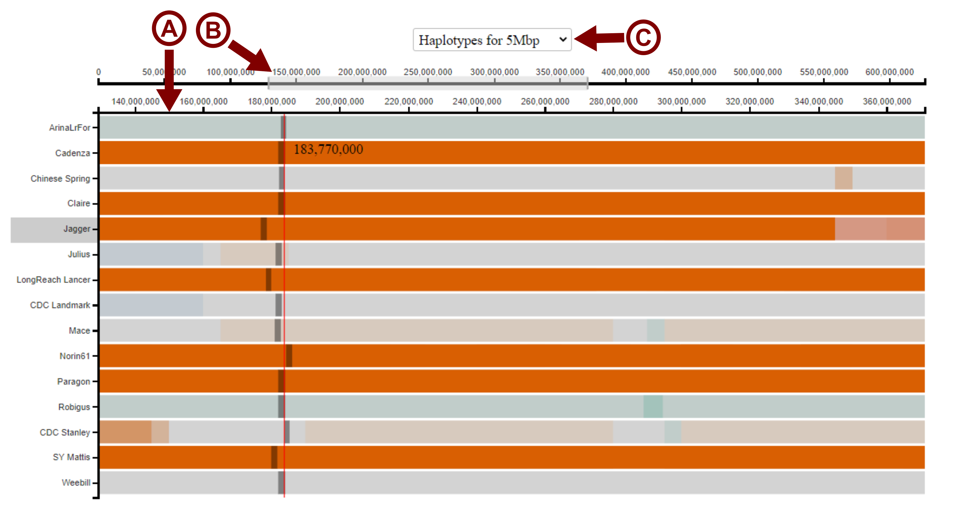
To zoom in on a particular region, the user can click and drag the cursor across the lower of the two x-axes to select the region of interest. The visualisation will then zoom in on this region, with the scale of the lower x-axis changing to reflect this (arrow A in image below). The master x-axis (upper) will display the whole length of the chromosome, with the selected region highighted (arrow B in image below). The user may drag this selected region across the master x-axis to move the window of view along the chromosome. The user can also change the size of the selected region to zoom in and out again. The user can also change the bin-size used to call the haplotype blocks using the drop down menu depending on the desired resolution (arrow C in the image below). The default bin-size shown is 5 Mbp.
Case studies
Below are some examples of the types of regions and genes that can be explored using the haplotype browser.
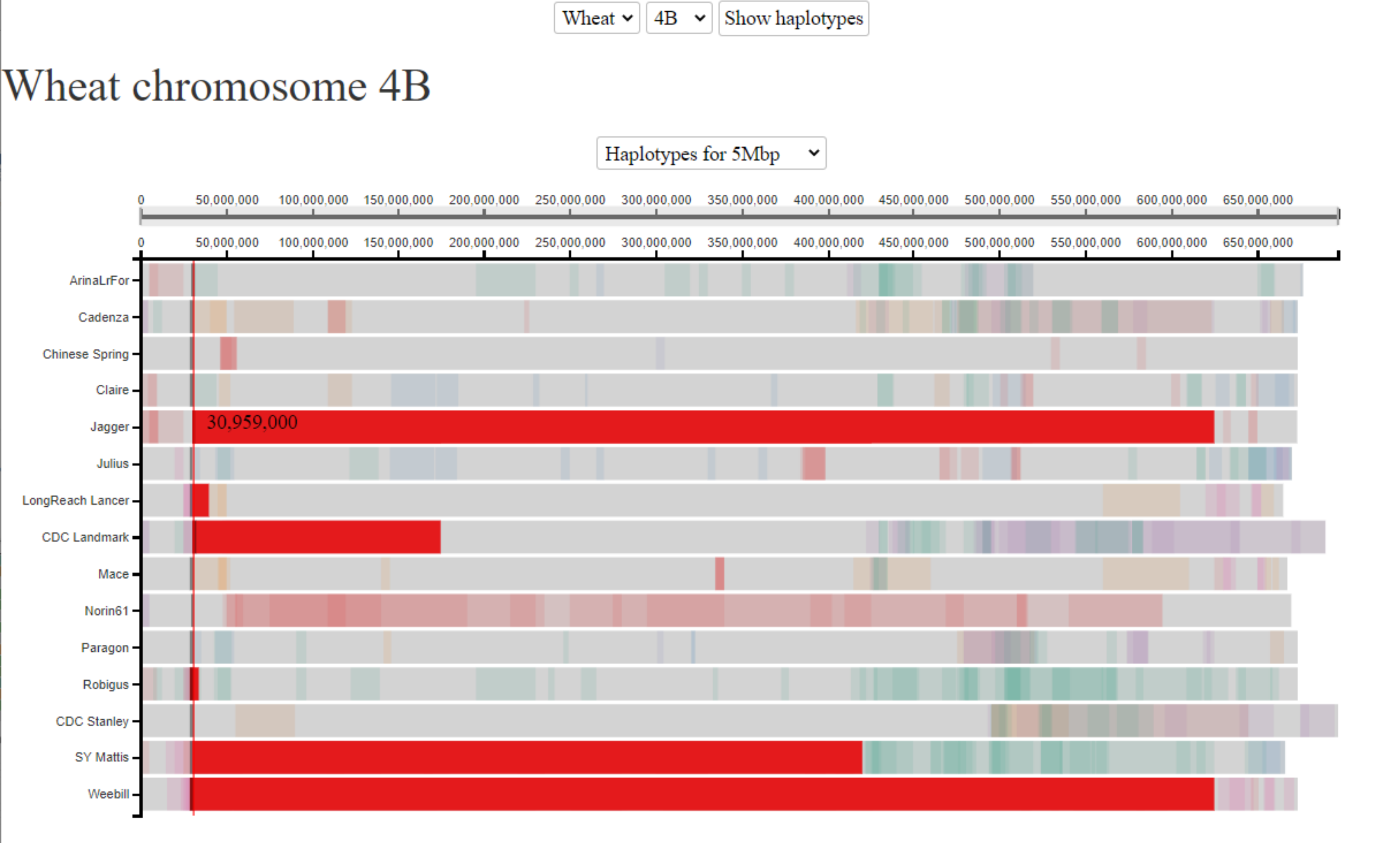
Example 1: Reduced Height (RHT-B1) gene
In this example, we are interested in understanding the haplotypes surrounding one of the Reduced Height genes, which were the genetic basis of the Green Revolution. We are interested in the Rht-B1 gene, which is located on chromosome 4B at ~30.6 Mbp. The Rht-B1b allele gives the reduced height phenotype and was introduced from a single source. We know that Jagger carries this allele. We therefore click on the gene location in Jagger and highlight shared haplotype blocks in 5 additional cultivars. All of these 5 additional cultivars are also known to carry the Rht-B1b allele, whilst all of the other cultivars carry WT alleles (different Rht-B1a alleles). The fact that all cultivars carrying the Rht-B1b allele have a shared haplotype at this position is consistent with the fact that the allele was introduced from a single source. Interestingly, the size of the shared haplotype block surrounding the Rht-B1b allele varies a great deal between the different cultivars, due to subsequent selection and recombination through breeding.
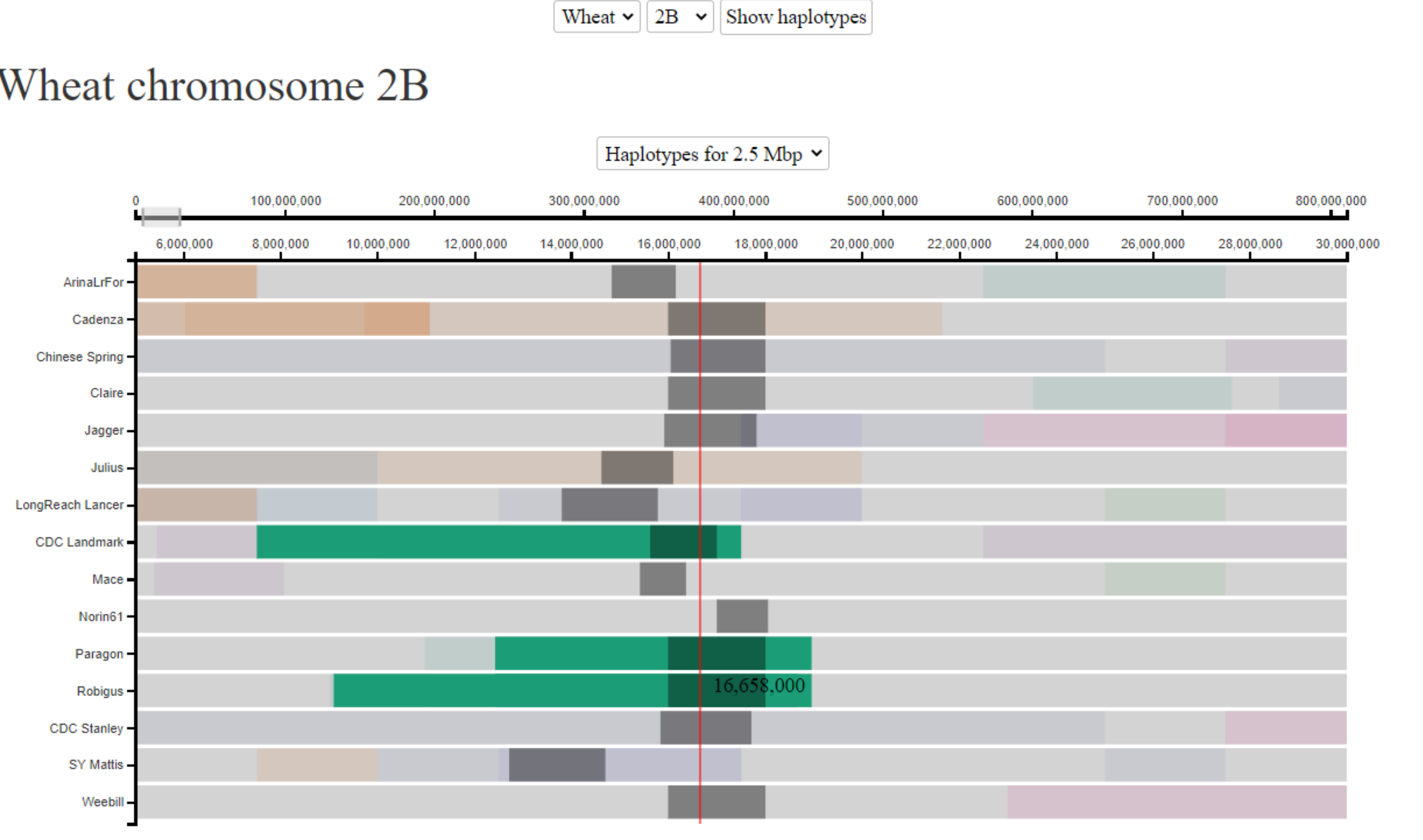
Example 2: Sm1 (Orange Wheat Blossom Midge (OWBM) resistance gene)
Cultivars Landmark, Robigus and Paragon are all known to be carriers of the Sm1 gene, which confers resistance to OWBM. We are interested to know whether all 3 cultivars obtained the resistance from the same source (i.e. do they share the same haplotype surrounding the gene). This is of particular interest given that the cultivars were developed through breeding programs in different countries (CDC Landmark - Canada, Robigus and Paragon - UK). The Sm1 gene is located on chromosome 2B at ~16 Mbp. In the below image we can see that CDC Landmark, Robigus and Paragon all share the same haplotype surrounding the Sm1 gene, suggesting that the resistance comes from a single source. In this case, the haplotype blocks are relatively small in size, so we have zoomed in and used the 2.5 Mbp bin-size to provide higher resolution.
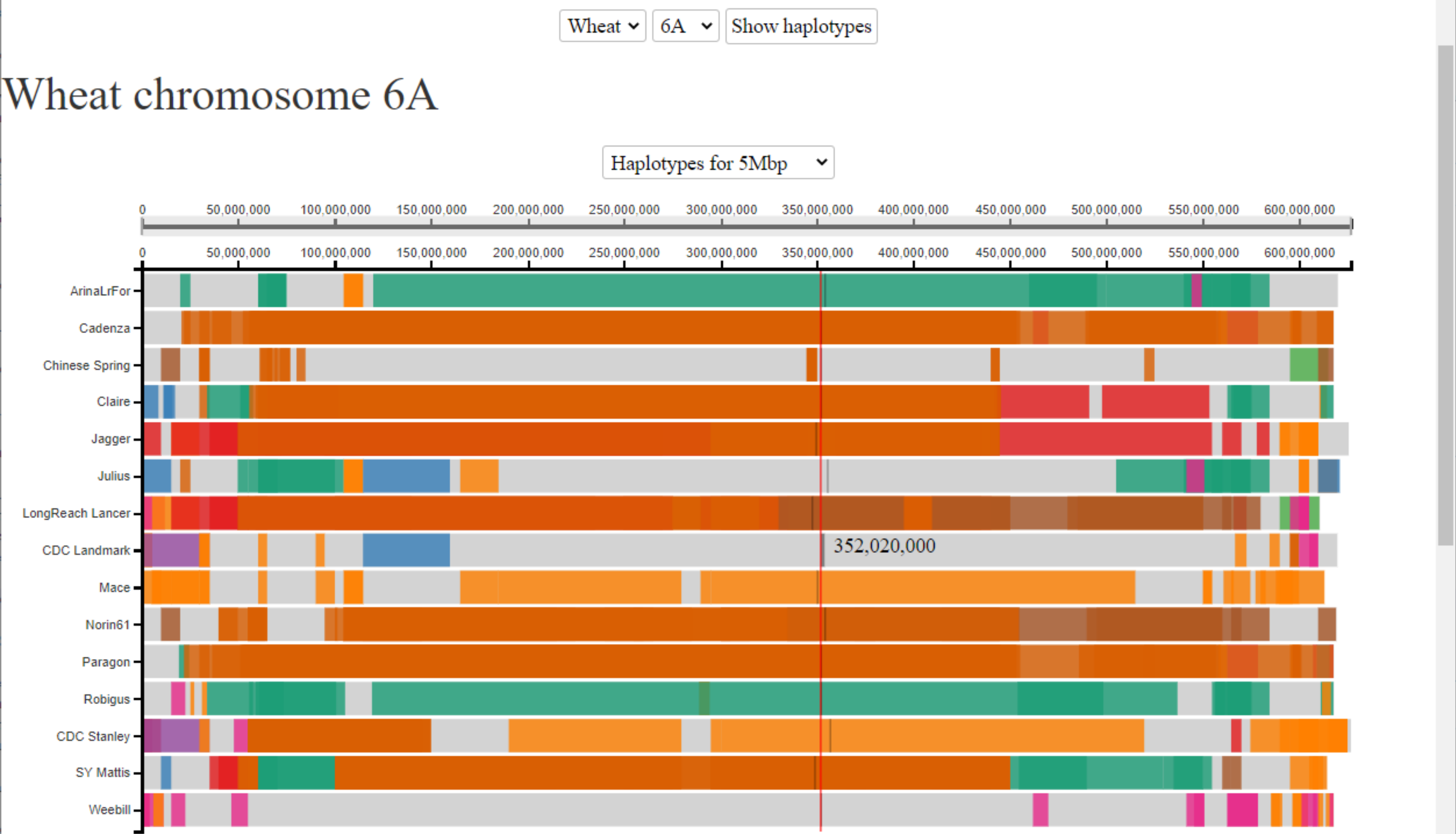
Example 3: Yield QTL on chromosome 6A
We are interested in a yield QTL that we identified in a mapping population between two UK wheat cultivars. The yield phenotype maps to an interval between 200-400 Mbp on chromosome 6A. We are interested to know how many haplotypes there are in this region in the 10+ genomes cultivars and how far these haplotype blocks extend. Here we see that we have seven different haplotypes across this region (3 shared amongst two or more cultivars (in orange, brown and green) and 4 unique to a single cultivar (light grey)). We can use this haplotype information to design genetic markers specific to each of the haplotype groups to determine whether either of our mapping parents share any of the haplotypes. If so, we can use the corresponding assemblies as proxy genome assemblies for our mapping parents to look at all of the genes lying in this region given that the genomic sequence will be identical-by-state.
For more details please see Brinton et al, 2020.
Example 4: Structural Rearrangement (inversion) on chromosome 3D
Structural rearrangements that occur on more than one cultivar may be of agronomic relevance. Here we exemplify how they can be detected in the browser with an example of an inversion. Cultivars CDC_Landmark and CDC_Stanley have an identical by state region (shown in orange/purple in the video below) that also contains an inversion from 441 to 510 Mbp with respect to Chinese Spring and all other pangenome assemblies. This information is revealed by the shadows that highlight corresponding blocks across the pangenome. We can observe in the video that the shadow starts at equivalent positions across all pangenome cultivars. By tracking CDC_Stanley (in orange), the shadow suddenly "jumps" to the end of the region with an inversion in all other cultivars (apart from CDC_Landmark). The same happens when we trace back the region in CDC_Landmark (in purple); as the shadow moves left in the two cultivars, it is moving in the opposite direction in all other cultivars. This exemplifies how we can identify structural variants, such as this inversion, based on the haplotype visualisation.
Contact
If you have suggestions of features that you would find useful and we could incorporate, please do not hesitate to get in touch with Ricardo Ramirez-Gonzalez and Cristobal Uauy.